Getting Started with multiGGM • multiGGM

Introduction

The multiGGM package implements the Bayesian method of Peterson, Stingo & Vannucci (2015, JASA) for joint inference of multiple Gaussian graphical models (GGMs). Given data from $K$ groups, the method simultaneously estimates group-specific precision matrices $\Omega_k$ and their associated conditional independence graphs $G_k$ , while borrowing strength across groups through a Markov random field (MRF) prior.

This vignette walks through:

Simulating multi-group data with known graph structure
Fitting the model with multiggm_mcmc()
Checking convergence
Extracting and interpreting results
Comparing estimated graphs to ground truth
Running and summarizing multiple MCMC chains

1. Simulate data

We generate data from two groups with $p = 15$ variables and $n = 100$ observations each, using a banded (AR-2) graph structure.

library(multiGGM)

sim <- simulate_multiggm(
  K = 2, p = 20, n = 100,
  graph_type = "random",
  perturb_prob = 0.1,
  seed = 42
)

cat("True edge counts:\n")
#> True edge counts:
for (k in 1:sim$K) {
  adj_k <- sim$adj_list[[k]]
  cat(sprintf("  Group %d: %d edges\n", k, sum(adj_k[upper.tri(adj_k)])))
}
#>   Group 1: 15 edges
#>   Group 2: 32 edges

2. Fit the model

We pass raw data matrices directly. The function computes cross-product matrices internally after column-centering.

fit <- multiggm_mcmc(
  data_list = sim$data_list,
  burnin = 200,
  nsave = 100,
  thin = 1,
  seed = 123
)

fit
#> <multiggm_fit>
#>   K groups: 2 
#>   p nodes : 20 
#>   Posterior draws: 100

3. Check convergence

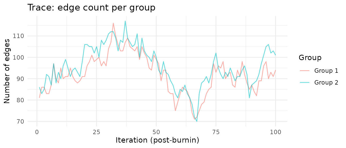
Summary

The summary() method reports acceptance rates and edge counts. Acceptance rates between 20-60% are generally healthy.

summary(fit, pip_threshold = .3)
#> multiGGM MCMC Summary
#> =====================
#> Groups (K): 2   |  Nodes (p): 20   |  Posterior draws: 100 
#> 
#> Acceptance rates:
#>   gamma (edge toggle): 1.0% 
#>   theta (within-model): 10.1% 
#>   nu (edge log-odds): 54.8% 
#> 
#> Selected edges (PIP >= 0.3 ):
#>   Group 1 : 128 edges
#>   Group 2 : 130 edges
#> 
#> Graph similarity (theta):
#>   theta[1,2]: mean = 1.264, P(nonzero) = 100.0%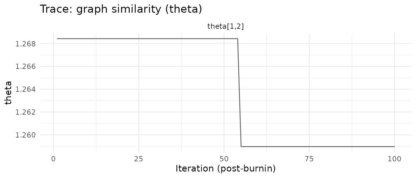

Trace plots

Trace plots help assess mixing. The theta trace shows the graph similarity parameter – values above zero indicate the model is borrowing strength across groups.

plot(fit, type = "trace_theta")

plot(fit, type = "trace_edges")

4. Extract results

Posterior inclusion probabilities (PIP)

PIPs indicate how often each edge was included across posterior samples. Higher PIP = stronger evidence for that edge.

pip <- pip_edges(fit)

plot(fit, type = "pip")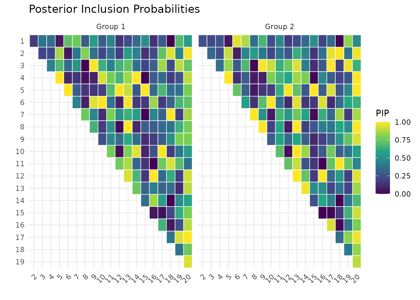

Estimated precision and partial correlations

The coef() method returns posterior mean precision matrices, while fitted() returns posterior mean partial correlations.

omega_hat <- coef(fit)
cat("Posterior mean precision (Group 1, first 5x5 block):\n")
#> Posterior mean precision (Group 1, first 5x5 block):
round(omega_hat[[1]][1:5, 1:5], 3)
#>        [,1]   [,2]   [,3]   [,4]  [,5]
#> [1,]  1.325 -0.010 -0.074 -0.053 0.013
#> [2,] -0.010  1.019 -0.001  0.025 0.109
#> [3,] -0.074 -0.001  1.124 -0.093 0.001
#> [4,] -0.053  0.025 -0.093  1.696 0.671
#> [5,]  0.013  0.109  0.001  0.671 1.413

pcor_hat <- fitted(fit)
cat("Posterior mean partial correlations (Group 1, first 5x5 block):\n")
#> Posterior mean partial correlations (Group 1, first 5x5 block):
round(pcor_hat[[1]][1:5, 1:5], 3)
#>        [,1]   [,2]   [,3]   [,4]   [,5]
#> [1,]  1.000  0.009  0.060  0.035 -0.009
#> [2,]  0.009  1.000  0.001 -0.018 -0.091
#> [3,]  0.060  0.001  1.000  0.064 -0.002
#> [4,]  0.035 -0.018  0.064  1.000 -0.432
#> [5,] -0.009 -0.091 -0.002 -0.432  1.000

Credible intervals

pcor_draws <- posterior_pcor(fit)
ci <- posterior_ci(pcor_draws)

# Example: 95% CI for edge (1,2) in group 1
cat(sprintf("pcor[1,2] Group 1: %.3f (%.3f, %.3f)\n",
            ci$median[1, 2, 1], ci$lower[1, 2, 1], ci$upper[1, 2, 1]))
#> pcor[1,2] Group 1: -0.000 (-0.026, 0.112)

5. Compare to ground truth

Visual comparison

plot_recovery() shows the true graph, PIP heatmap, and thresholded estimate side-by-side.

cm <- plot_recovery(fit, sim$adj_list, pip_threshold = 0.5)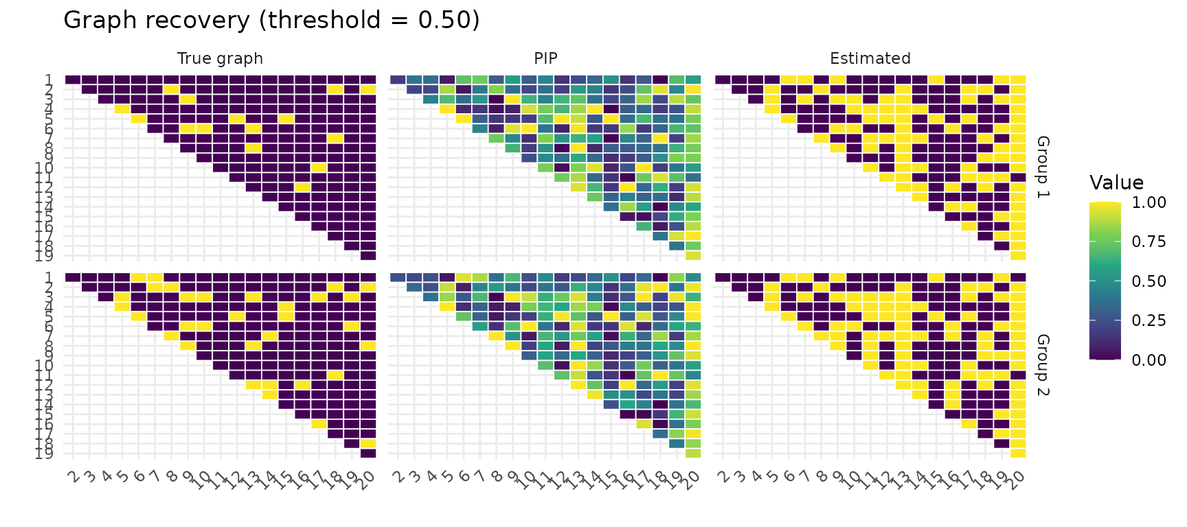

Confusion metrics

for (k in seq_along(cm)) {
  cat(sprintf("Group %d: TP=%d, FP=%d, FN=%d, TN=%d, TPR=%.2f, FPR=%.2f\n",
              k, cm[[k]]["TP"], cm[[k]]["FP"], cm[[k]]["FN"], cm[[k]]["TN"],
              cm[[k]]["TPR"], cm[[k]]["FPR"]))
}
#> Group 1: TP=15, FP=70, FN=0, TN=105, TPR=1.00, FPR=0.40
#> Group 2: TP=30, FP=59, FN=2, TN=99, TPR=0.94, FPR=0.37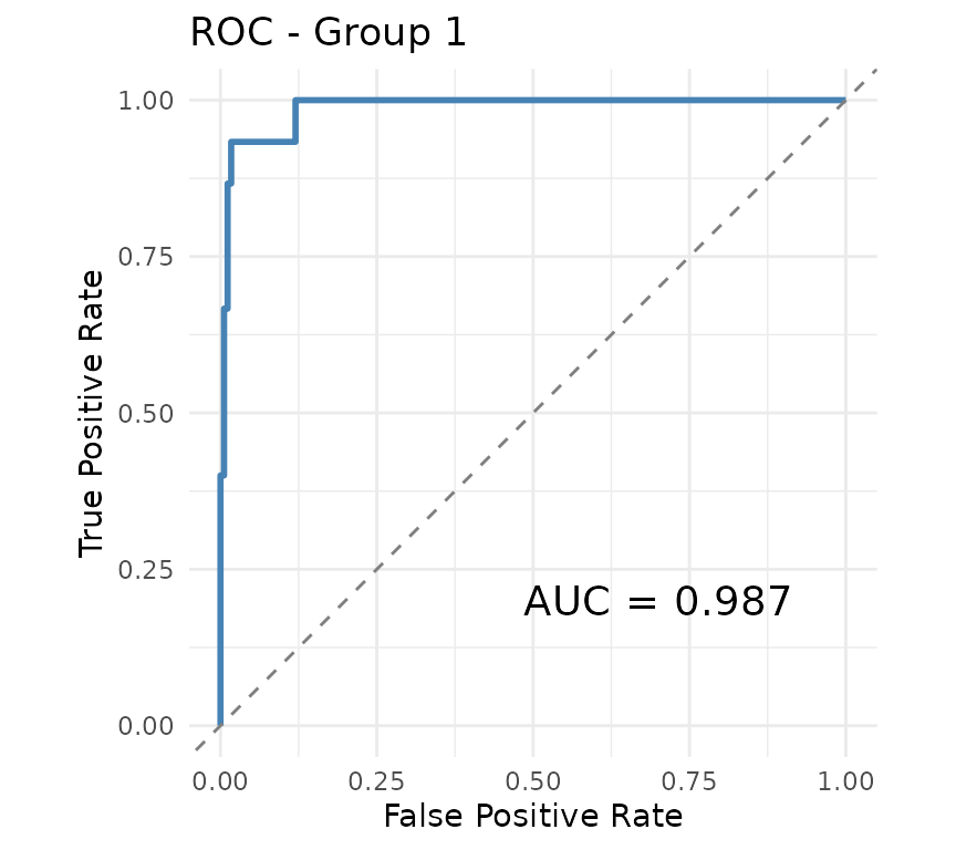

ROC curve

The ROC curve evaluates edge selection across all possible thresholds.

roc1 <- roc_auc(pip[, , 1], sim$adj_list[[1]])
plot_roc(roc1, main = "ROC - Group 1")

6. Network visualization

We can visualize the estimated graph as a network.

par(mfrow = c(1, 2))
plot_network(sim$adj_list[[1]], main = "True - Group 1", vertex_size = 12)
est_adj <- (pip[, , 1] >= 0.3) * 1L
plot_network(est_adj, main = "Estimated - Group 1", vertex_size = 12)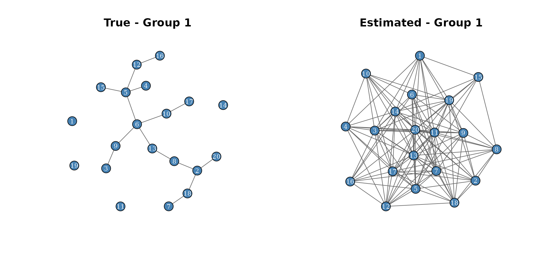

7. Differential edges

For $K = 2$ groups, we can identify edges that differ between groups.

pip_diff <- pip_diff_edge(fit)
cat("Edges with P(differential) > 0.5:",
    sum(pip_diff[upper.tri(pip_diff)] > 0.5), "\n")
#> Edges with P(differential) > 0.5: 0

pcor_draws <- posterior_pcor(fit)
diff_prob <- diff_prob_pcor(pcor_draws, delta = 0.1)
cat("Edges with P(|pcor diff| > 0.1) > 0.5:",
    sum(diff_prob[upper.tri(diff_prob)] > 0.5), "\n")
#> Edges with P(|pcor diff| > 0.1) > 0.5: 56

8. Running multiple chains

Running multiple MCMC chains from different starting points is important for assessing convergence. The multiggm_mcmc() function supports this via the nchains argument. Chains can be run in parallel with parallel = TRUE.

Fitting multiple chains

fit_mc <- multiggm_mcmc(
  data_list = sim$data_list,
  burnin    = 2000,
  nsave     = 1000,
  nchains   = 3,
  parallel  = TRUE,
  seed      = 42
)

The result is a multiggm_fit_list object containing all chains:

fit_mc
#> <multiggm_fit_list>
#>   Chains: 3 
#>   K groups: 2

Accessing individual chains

Each chain is a full multiggm_fit object. Access them via $chains:

# Summary of chain 1
summary(fit_mc$chains[[1]], pip_threshold = 0.3)
#> multiGGM MCMC Summary
#> =====================
#> Groups (K): 2   |  Nodes (p): 20   |  Posterior draws: 1000 
#> 
#> Acceptance rates:
#>   gamma (edge toggle): 0.2% 
#>   theta (within-model): 3.6% 
#>   nu (edge log-odds): 61.7% 
#> 
#> Selected edges (PIP >= 0.3 ):
#>   Group 1 : 186 edges
#>   Group 2 : 186 edges
#> 
#> Graph similarity (theta):
#>   theta[1,2]: mean = 1.868, P(nonzero) = 100.0%

Most utility functions accept a chain argument to select which chain to analyze:

# PIPs from chain 1 vs chain 2
pip_c1 <- pip_edges(fit_mc, chain = 1)
pip_c2 <- pip_edges(fit_mc, chain = 2)

idx <- upper.tri(pip_c1[, , 1])
cat(sprintf("PIP correlation between chain 1 and 2 (Group 1): %.3f\n",
            cor(pip_c1[, , 1][idx], pip_c2[, , 1][idx])))
#> PIP correlation between chain 1 and 2 (Group 1): 0.832

Comparing trace plots across chains

Overlaying trace plots from multiple chains is one of the most effective visual convergence diagnostics. Chains that have converged will mix and overlap, while chains stuck in different modes will show persistent separation.

library(ggplot2)

# Build a combined edge-count trace from all chains
trace_df <- do.call(rbind, lapply(seq_len(fit_mc$nchains), function(ch) {
  ec <- edge_counts(fit_mc, chain = ch)
  data.frame(
    iteration = seq_len(nrow(ec)),
    edges     = ec[, 1],
    chain     = paste("Chain", ch),
    stringsAsFactors = FALSE
  )
}))

ggplot(trace_df, aes(x = iteration, y = edges, color = chain)) +
  geom_line(alpha = 0.6) +
  labs(title = "Edge count trace (Group 1) across chains",
       x = "Iteration (post-burnin)", y = "Number of edges") +
  theme_minimal()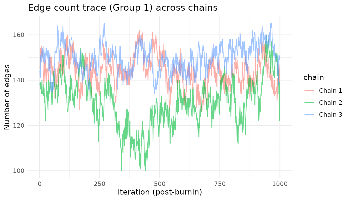

# Overlay theta traces from all chains
theta_df <- do.call(rbind, lapply(seq_len(fit_mc$nchains), function(ch) {
  data.frame(
    iteration = seq_len(dim(fit_mc$chains[[ch]]$Theta_save)[3]),
    theta     = fit_mc$chains[[ch]]$Theta_save[1, 2, ],
    chain     = paste("Chain", ch),
    stringsAsFactors = FALSE
  )
}))

ggplot(theta_df, aes(x = iteration, y = theta, color = chain)) +
  geom_line(alpha = 0.6) +
  labs(title = "Trace: theta[1,2] across chains",
       x = "Iteration (post-burnin)", y = "theta[1,2]") +
  theme_minimal()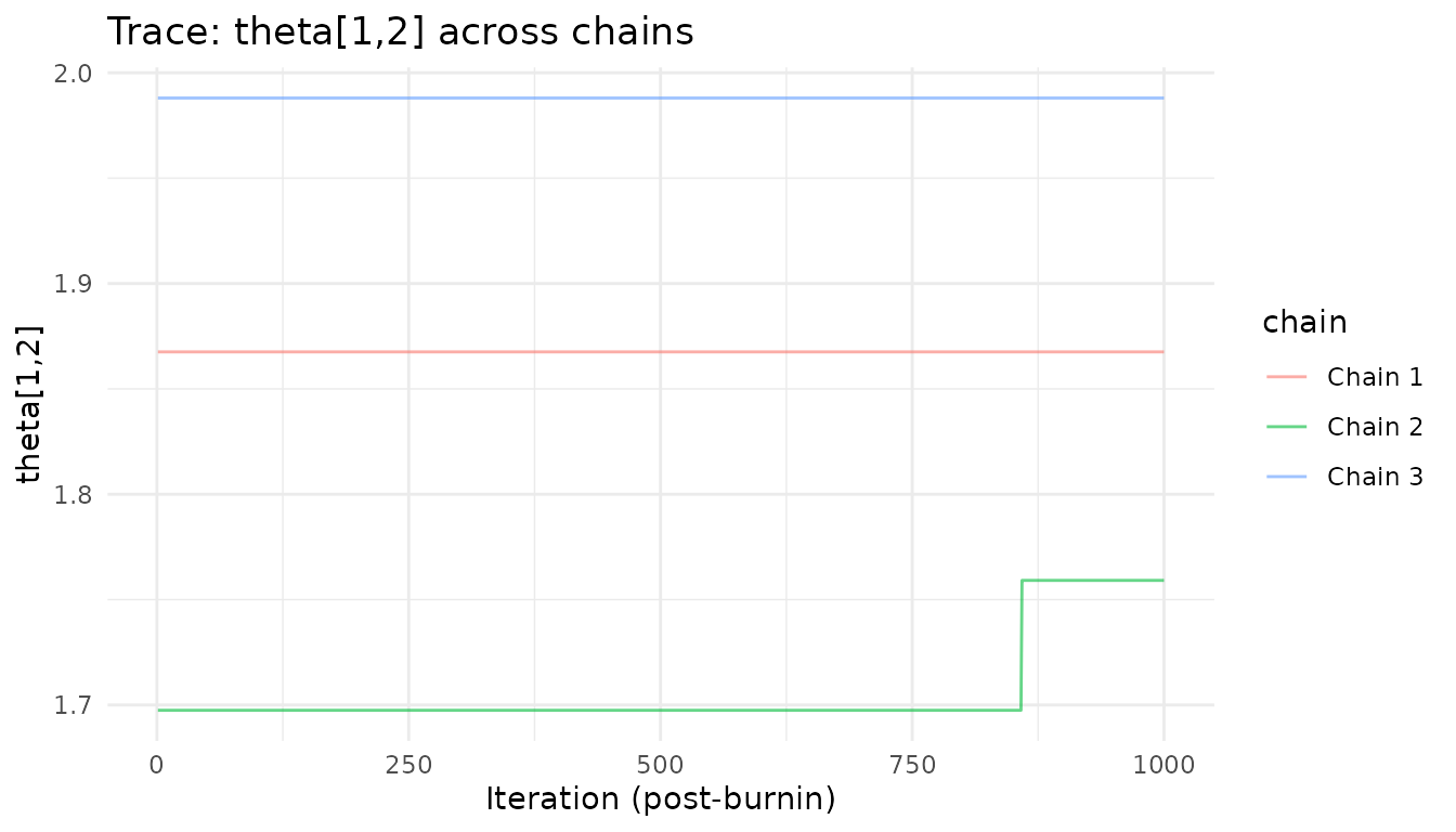

Pooling results across chains

To combine posterior samples from all chains, concatenate the saved arrays along the iteration dimension:

# Pool precision draws across all chains
pool_C <- abind::abind(
  lapply(fit_mc$chains, function(ch) ch$C_save),
  along = 4
)
cat(sprintf("Pooled draws: %d (from %d chains x %d draws each)\n",
            dim(pool_C)[4], fit_mc$nchains, dim(fit_mc$chains[[1]]$C_save)[4]))
#> Pooled draws: 3000 (from 3 chains x 1000 draws each)

# Pool adjacency draws for combined PIPs
pool_adj <- abind::abind(
  lapply(fit_mc$chains, function(ch) ch$adj_save),
  along = 4
)
pip_pooled <- apply(pool_adj, c(1, 2, 3), mean)

cat(sprintf("Pooled edges (PIP > 0.5, Group 1): %d\n",
            sum(pip_pooled[, , 1][upper.tri(pip_pooled[, , 1])] > 0.5)))
#> Pooled edges (PIP > 0.5, Group 1): 170

Summary of multi-chain functions

Task	Code
Fit multiple chains	`multiggm_mcmc(..., nchains = 4, parallel = TRUE)`
Access chain $i$	`fit$chains[[i]]`
PIPs from chain $i$	`pip_edges(fit, chain = i)`
Partial correlations from chain $i$	`posterior_pcor(fit, chain = i)`
Precision matrices from chain $i$	`posterior_precision(fit, chain = i)`
Edge counts from chain $i$	`edge_counts(fit, chain = i)`
Pool draws across chains	`abind::abind(lapply(fit$chains, \(ch) ch$C_save), along = 4)`

References

Peterson, C.B., Stingo, F.C. & Vannucci, M. (2015). Bayesian inference of multiple Gaussian graphical models. Journal of the American Statistical Association, 110(509), 159-174.