Scalable Inference with the SSVS Method

Overview

Version 0.2.0 of multiGGM adds a second inference method: the spike-and-slab continuous shrinkage prior of Shaddox et al. (2018, Statistics in Biosciences). This method replaces the G-Wishart prior and Wang-Li exchange algorithm with a column-wise Gibbs sampler that scales to graphs with $p > 100$ nodes.

Select the method via the method argument:

# Original G-Wishart method (default, best for small p)
fit_gw <- multiggm_mcmc(data_list, method = "gwishart")

# Scalable SSVS method (for larger p)
fit_ssvs <- multiggm_mcmc(data_list, method = "ssvs")

Both methods estimate the same quantities—group-specific precision matrices $\Omega_k$, adjacency matrices $G_k$, graph similarity parameters $\theta_{km}$, and edge-specific log-odds $\nu_{ij}$—and the output objects have an identical structure. All post-processing functions (pip_edges, posterior_pcor, plot, etc.) work with either method.

When to use each method

Scenario	Recommended method
$p \le 30$, need exact G-Wishart inference	"gwishart"
$p > 30$, exploratory analysis	"ssvs"
$p > 50$, any use case	"ssvs" (G-Wishart becomes prohibitively slow)
Comparing both priors on the same data	Run both, compare PIPs

Quick start example

library(multiGGM)

sim <- simulate_multiggm(K = 2, p = 30, n = 100, seed = 42)

fit <- multiggm_mcmc(
  data_list = sim$data_list,
  method    = "ssvs",
  burnin    = 200,
  nsave     = 100,
  seed      = 123
)

# TODO add section on multiple chains, how to use them and how to evaluate convergence, and when it is recommended to use more than one chain

summary(fit, pip_threshold = 0.5)
#> multiGGM MCMC Summary
#> =====================
#> Groups (K): 2   |  Nodes (p): 30   |  Posterior draws: 100 
#> 
#> Acceptance rates:
#>   gamma (edge toggle): 24.0% 
#>   theta (within-model): 2.3% 
#>   nu (edge log-odds): 43.2% 
#> 
#> Selected edges (PIP >= 0.5 ):
#>   Group 1 : 14 edges
#>   Group 2 : 14 edges
#> 
#> Graph similarity (theta):
#>   theta[1,2]: mean = 0.009, P(nonzero) = 9.0%

plot(fit, type = "pip")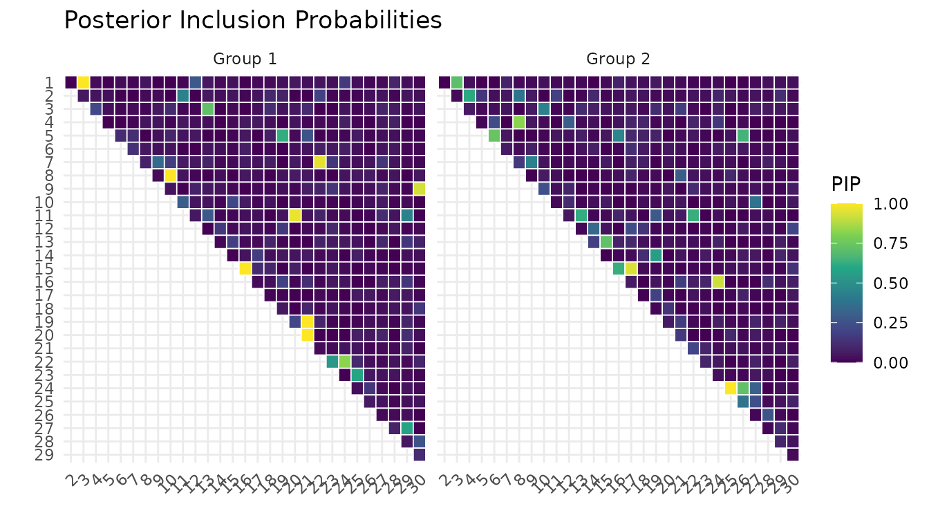

plot(fit, type = "trace_theta")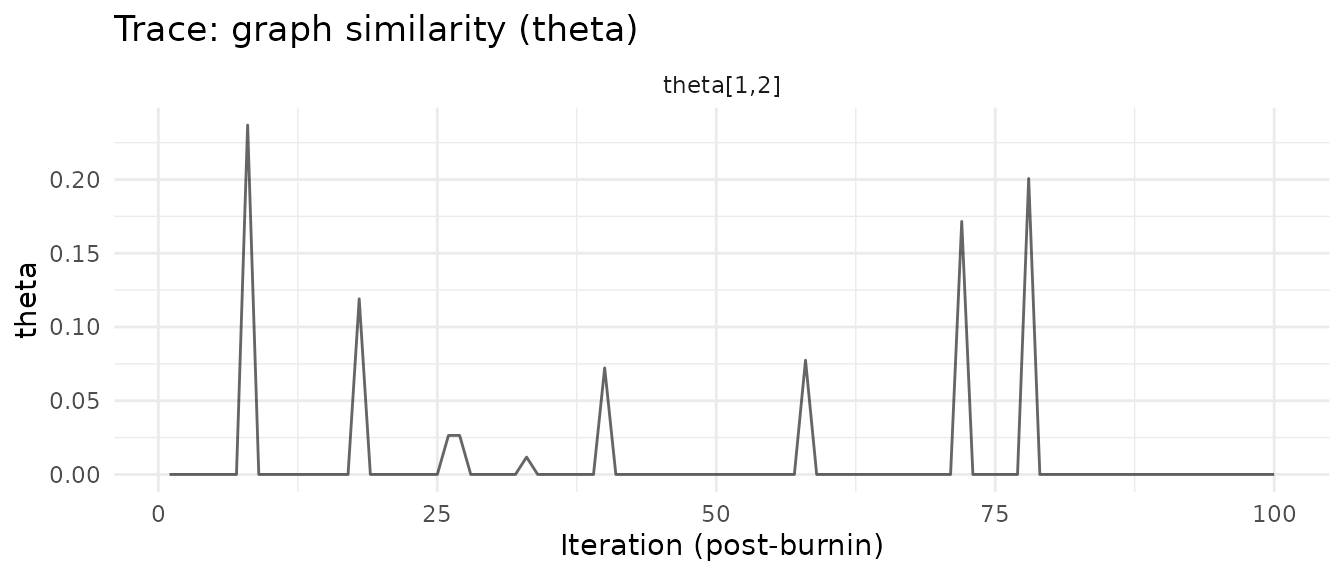

Scalability benchmarks

The table below shows wall-clock times for 200 burn-in + 100 saved iterations with $K = 2$ groups and $n = 100$ observations per group, measured on an Apple M1 processor.

$p$	SSVS	G-Wishart	Speedup
10	0.1 s	0.8 s	6x
20	0.7 s	10.9 s	17x
30	1.7 s	104.9 s	63x
50	7.5 s	(infeasible)	—

The speedup increases with $p$ because the G-Wishart method’s cost grows as $O(K \cdot p^4)$ per iteration (due to per-edge exchange proposals and BIPS clique updates), while the SSVS method grows as $O(K \cdot p^3)$ (column-wise Gibbs sweeps with rank-1 covariance updates).

How the two methods differ

Both methods share the same Markov random field (MRF) prior that borrows strength across groups, and the same Metropolis-Hastings updates for the graph similarity parameters $\theta_{km}$ and edge-specific log-odds $\nu_{ij}$. They differ only in how the precision matrices $\Omega_k$ and graphs $G_k$ are sampled.

G-Wishart method (method = "gwishart")

The original Peterson et al. (2015) approach places a G-Wishart prior $\Omega_k \mid G_k \sim W_G(b, D)$ on each precision matrix. Sampling proceeds via the Wang-Li (2012) exchange algorithm:

• For each edge $(i,j)$ in each group $k$:
  1. Compute a Bernoulli proposal probability from the G-Wishart posterior ratio (log_H) and the MRF similarity term.
  2. If the proposed graph differs, sample a new precision matrix from the G-Wishart conditional (GWishart_NOij_Gibbs).
  3. Accept or reject via an exchange ratio involving G-Wishart pdf evaluations (log_GWishart_NOij_pdf).
  4. Update the precision matrix from the posterior conditional.
• After all edges: refresh the full precision matrix via BIPS (Block Incomplete Partial correlation Sampling) using maximal clique decomposition (GWishart_BIPS_maximumClique).

This requires $O(p^2)$ edge proposals per group, each involving $O(p^2)$–$O(p^3)$ matrix operations, plus an additional $O(p^2)$ BIPS step.

SSVS method (method = "ssvs")

The Shaddox et al. (2018) approach replaces the G-Wishart prior with a spike-and-slab normal prior on each off-diagonal precision element:

$$\omega_{k,ij} \mid z_{k,ij} \sim (1 - z_{k,ij}) \cdot N(0, v_0) + z_{k,ij} \cdot N(0, v_1)$$

where $v_0 \ll v_1$ (spike vs. slab), and an exponential prior on diagonal elements: $\omega_{k,ii} \sim \text{Exp}(\lambda/2)$. Because this prior has a tractable normalizing constant, sampling uses a direct column-wise Gibbs sweep:

• For each column $i$ of the precision matrix in each group $k$:
  1. Compute the Schur complement $C_{11}^{-1} = \Sigma_{11} - \Sigma_{12}\Sigma_{12}^\top / \Sigma_{ii}$ from the current covariance (no matrix inversion needed).
  2. Form the posterior precision $C_i = (S_{ii} + \lambda) \cdot C_{11}^{-1} + \text{diag}(1/\tau)$, where $\tau$ contains $v_0$ or $v_1$ depending on current edge inclusion.
  3. Sample the off-diagonal column from its multivariate normal conditional: $\epsilon \sim N(\mu_i, C_i^{-1})$.
  4. Sample the diagonal from a Gamma conditional: $\gamma \sim \text{Gamma}(n_k/2 + 1,\; (S_{ii} + \lambda)/2)$.
  5. Rank-1 covariance update: update $\Sigma$ directly from the new column without any full matrix inversion.
  6. Update edge indicators $z$ via posterior spike-slab odds, incorporating the MRF prior analytically through the conditional inclusion probability.

There is no exchange algorithm, no BIPS clique step, and no trans-dimensional moves. Each iteration costs $O(p)$ column sweeps, each $O(p^2)$ for the Cholesky solve and rank-1 update, giving $O(p^3)$ total per group per iteration.

What stays the same

• The MRF normalizing constant $C(\theta, \nu_{ij})$ uses the same exact enumeration over $\{0,1\}^K$ binary vectors (feasible when $K$ is small).
• The $\theta_{km}$ update (between-model spike/slab toggle + within-model Gamma proposal) and the $\nu_{ij}$ update (MH with Beta proposal) are identical in both methods.

Key differences at a glance

Aspect	G-Wishart	SSVS
Precision prior	G-Wishart $W_G(b, D)$	Spike-slab $N(0, v_0)$ / $N(0, v_1)$
Graph sampling	Exchange algorithm (MH per edge)	Posterior Bernoulli from spike-slab odds
Precision sampling	NOij Gibbs per edge + BIPS clique	Column-wise Gaussian conditional
Covariance updates	Full inversion after BIPS	Rank-1 incremental update
Complexity/iter	$O(K \cdot p^4)$	$O(K \cdot p^3)$
Scalability	$p \lesssim 30\text{--}50$	$p > 100$ demonstrated

SSVS hyperparameters

Default values

The SSVS-specific hyperparameters and their defaults are:

Parameter	Default	Role
v0	$0.02^2 = 0.0004$	Spike variance (small, effectively zeroes the edge)
v1	$50^2 \times v_0 = 1.0$	Slab variance (large, allows substantial precision values)
lambda	1	Exponential rate for diagonal elements

The variance inflation ratio $h = v_1 / v_0 = 2500$ controls edge selection sensitivity. The prior edge inclusion probability adapts to the dimension: $\pi = 2/(p-1)$, which favors sparse graphs as $p$ grows.

These defaults follow Wang (2015, Bayesian Analysis), “Scaling it up: stochastic search structure learning in graphical models,” which introduced the SSVS approach for single GGMs. The multiGGM implementation extends it to multiple graphs by adding MRF-coupled edge indicators.

Common hyperparameters (shared with G-Wishart)

Parameter	Default	Role
a, b	1, 4	Beta(1, 4) prior on edge inclusion log-odds $\nu_{ij}$; gives prior $P(\text{edge}) \approx 0.20$
alpha, beta	2, 5	Gamma(2, rate=5) slab prior on $\theta_{km}$; mean = 0.4
w	0.9	$P(\gamma_{km} = 1)$; strong prior belief that groups share structure
alpha_prop, beta_prop	1, 1	Gamma proposal for $\theta_{km}$ MH step (scale parameterization)

Tuning recommendations

• v0 and v1: The defaults work well for standardized data. If your data are on a very different scale, you may need to adjust. A larger v1 allows stronger partial correlations; a smaller v0 provides stricter edge selection.
• lambda: Controls diagonal shrinkage. The default of 1 is generally safe. Increasing lambda adds regularization to the diagonal.
• burnin and nsave: The SSVS sampler typically mixes faster than G-Wishart, so you may need fewer iterations. Start with burnin = 5000, nsave = 5000 and check trace plots. For production runs, Shaddox et al. (2018) used burnin = 40000, nsave = 80000.
• a and b: Decrease b for denser graphs (e.g., Beta(1, 1) for uniform prior on edge probability) or increase for sparser graphs (e.g., Beta(1, 9) for $$10% prior edge probability).

Passing custom hyperparameters

fit <- multiggm_mcmc(
  data_list = sim$data_list,
  method    = "ssvs",
  hyper     = list(
    v0    = 0.01^2,    # tighter spike
    v1    = 100^2 * 0.01^2,  # wider slab
    lambda = 2,        # stronger diagonal shrinkage
    a = 1, b = 9,      # sparser prior (Beta(1,9))
    alpha = 2, beta = 5,
    w = 0.5,           # less certain groups are related
    alpha_prop = 1, beta_prop = 1
  ),
  burnin = 5000,
  nsave  = 5000,
  seed   = 42
)

Comparing both methods on the same data

When $p$ is small enough to run both, comparing results provides a useful robustness check.

sim_small <- simulate_multiggm(K = 2, p = 15, n = 100, seed = 42, graph_type = "hub")

fit_gw <- multiggm_mcmc(
  data_list = sim_small$data_list,
  method    = "gwishart",
  burnin    = 2000,
  nsave     = 1000,
  seed      = 123
)

fit_ssvs <- multiggm_mcmc(
  data_list = sim_small$data_list,
  method    = "ssvs",
  hyper = list(
  v0    = 0.001,   
    v1    = 1,  
    lambda = 1,       
    a = 1, b = 4,    
    alpha = 2, beta = 5,
    w = 0.9,           # less certain groups are related
    alpha_prop = 1, beta_prop = 1),
  burnin    = 2000,
  nsave     = 1000,
  seed      = 123
)

pip_gw   <- pip_edges(fit_gw)
pip_ssvs <- pip_edges(fit_ssvs)

# Compare PIPs for group 1 (upper triangle only)
idx <- upper.tri(pip_gw[, , 1])
cat(sprintf("Correlation of PIPs (Group 1): %.3f\n",
            cor(pip_gw[, , 1][idx], pip_ssvs[, , 1][idx])))
#> Correlation of PIPs (Group 1): 0.930
cat(sprintf("G-Wishart edges (PIP > 0.5):   %d\n",
            sum(pip_gw[, , 1][idx] > 0.5)))
#> G-Wishart edges (PIP > 0.5):   14
cat(sprintf("SSVS edges (PIP > 0.5):        %d\n",
            sum(pip_ssvs[, , 1][idx] > 0.5)))
#> SSVS edges (PIP > 0.5):        10

Recovery comparison

par(mfrow = c(2, 1))
cm_gw   <- plot_recovery(fit_gw,   sim_small$adj_list, pip_threshold = 0.5)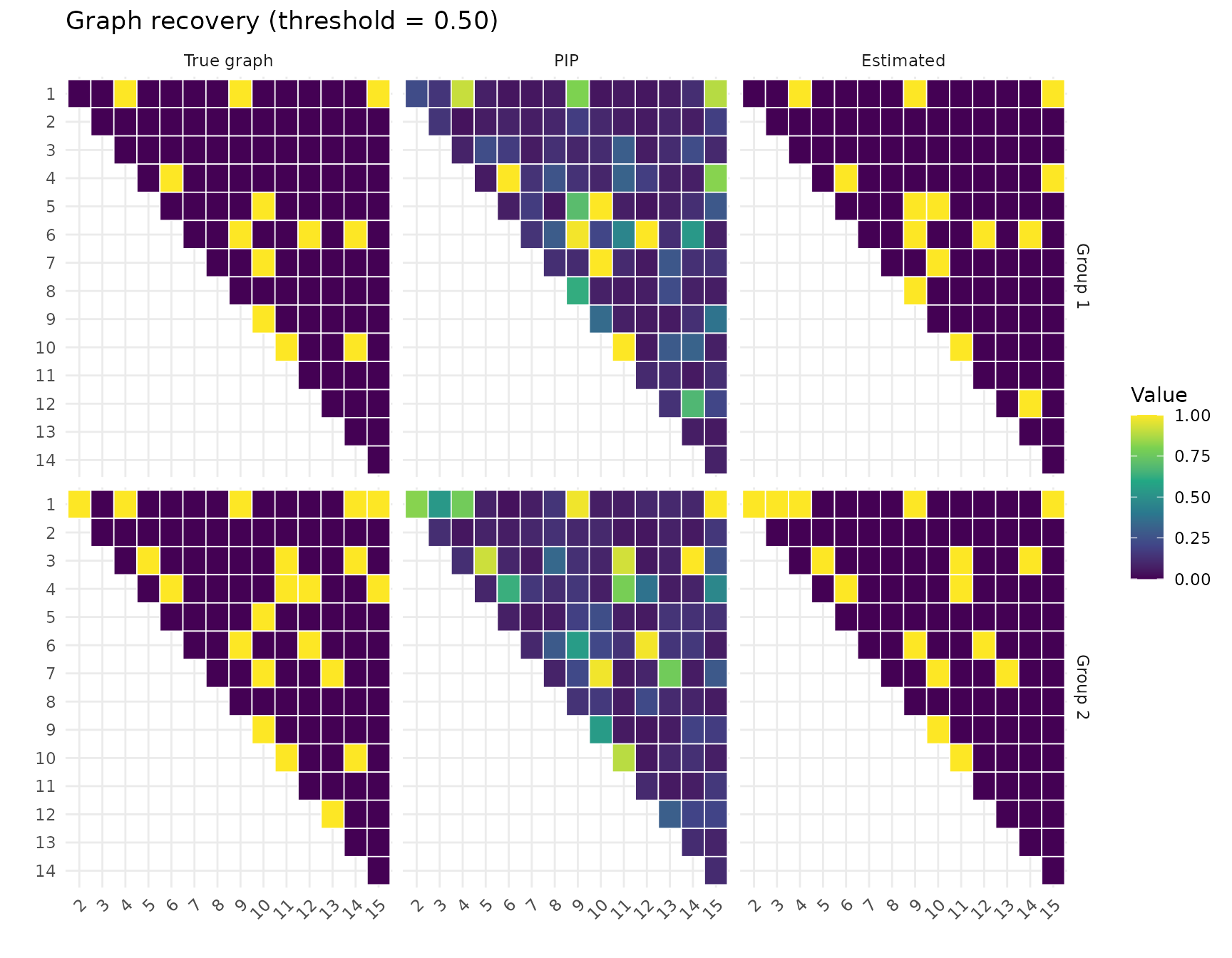

cm_ssvs <- plot_recovery(fit_ssvs, sim_small$adj_list, pip_threshold = 0.3)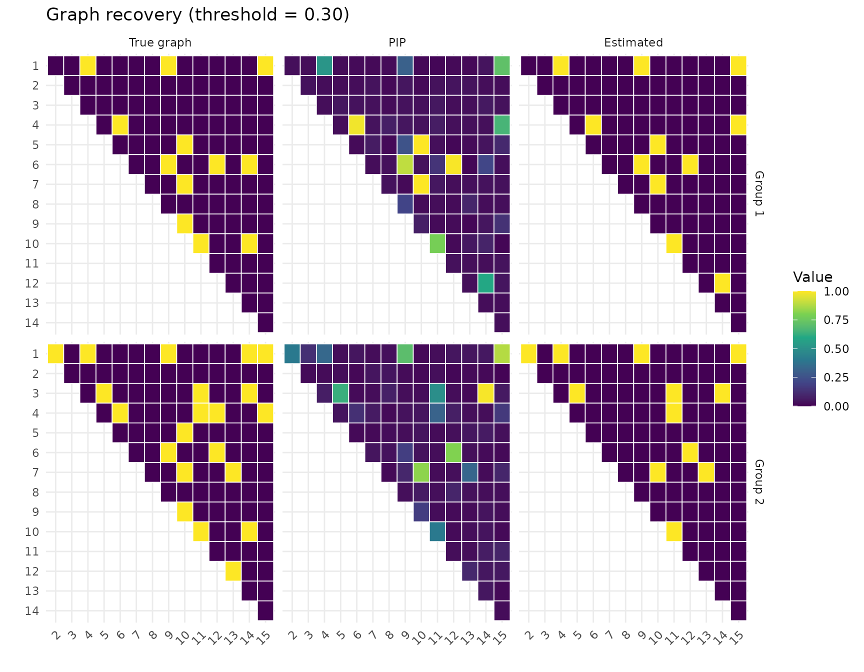

for (method_name in c("G-Wishart", "SSVS")) {
  cm <- if (method_name == "G-Wishart") cm_gw else cm_ssvs
  for (k in seq_along(cm)) {
    cat(sprintf("%s Group %d: TPR=%.2f, FPR=%.2f\n",
                method_name, k, cm[[k]]["TPR"], cm[[k]]["FPR"]))
  }
}
#> G-Wishart Group 1: TPR=0.83, FPR=0.04
#> G-Wishart Group 2: TPR=0.71, FPR=0.01
#> SSVS Group 1: TPR=0.75, FPR=0.02
#> SSVS Group 2: TPR=0.57, FPR=0.00

Running multiple chains

Both methods support running multiple independent MCMC chains for convergence assessment. Because the SSVS method is faster per iteration, running multiple chains is more practical at larger dimensions:

fit_mc <- multiggm_mcmc(
  data_list = sim$data_list,
  method    = "ssvs",
  burnin    = 2000,
  nsave     = 1000,
  nchains   = 3,
  parallel  = TRUE,
  seed      = 42
)

# Compare PIPs across chains to check convergence
pip_c1 <- pip_edges(fit_mc, chain = 1)
pip_c2 <- pip_edges(fit_mc, chain = 2)
pip_c3 <- pip_edges(fit_mc, chain = 3)

idx <- upper.tri(pip_c1[, , 1])
cat(sprintf("PIP correlation (chains 1-2): %.3f\n",
            cor(pip_c1[, , 1][idx], pip_c2[, , 1][idx])))
#> PIP correlation (chains 1-2): 0.970
cat(sprintf("PIP correlation (chains 1-3): %.3f\n",
            cor(pip_c1[, , 1][idx], pip_c3[, , 1][idx])))
#> PIP correlation (chains 1-3): 0.954

See the Getting Started vignette for a complete walkthrough of multi-chain diagnostics, including overlaid trace plots and pooling results across chains.

References

Peterson, C.B., Stingo, F.C. & Vannucci, M. (2015). Bayesian inference of multiple Gaussian graphical models. Journal of the American Statistical Association, 110(509), 159–174.

Shaddox, E., Stingo, F.C., Peterson, C.B., et al. (2018). A Bayesian approach for learning gene networks underlying disease severity in COPD. Statistics in Biosciences, 10(1), 59–85.

Wang, H. (2015). Scaling it up: stochastic search structure learning in graphical models. Bayesian Analysis, 10(2), 351–377.

Wang, H. & Li, S.Z. (2012). Efficient Gaussian graphical model determination under G-Wishart prior distributions. Electronic Journal of Statistics, 6, 168–198.