The Multiple Graphical Horseshoe (mGHS) • multiGGM

Overview

method = "mghs" fits the multiple graphical horseshoe of Busatto & Stingo (2025, JCGS). The sampler is adapted from the authors’ code (github.com/cbusatto/mGHS) and reproduces its draws exactly for the same seed. Local fixes and the validation are documented in system.file("mghs", package = "multiGGM").

Continuous shrinkage versus spike-and-slab

The G-Wishart ("gwishart") and SSVS ("ssvs") samplers have a binary indicator $g_{k,ij}$ for every edge. Each draw says which edges are in each graph, so the package can report posterior inclusion probabilities (pip_edges()) and the probability that an edge is in one graph but not the other (pip_diff_edge()). Groups borrow strength through an MRF prior on those indicators.

The mGHS has no indicators. Each precision entry $\omega_{k,ij}$ gets a horseshoe prior with a global scale $\tau_k$ and a local scale $\lambda_{ij,k}$ . Small entries are shrunk strongly towards zero but are never exactly zero. Groups borrow strength through a $K \times K$ correlation matrix $R$ that correlates each edge’s local scales across groups. $R = I$ gives independent graphical horseshoes.

So for mGHS fits:

pip_edges(), pip_diff_edge(), edge_counts() and the plots built on them stop with an error, rather than returning a number with a different meaning.
Edge strength comes from the posterior of the precision matrix or partial correlations (coef(), fitted(), posterior_pcor(), posterior_ci()).
Differential edges come from the posterior of the group difference $D_{ij} = \rho_{1,ij} - \rho_{2,ij}$ (diff_summary(), select_diff_edges()).

Fitting

library(multiGGM)
sim <- simulate_multiggm(K = 2, p = 12, n = 60, perturb_prob = 0.2, seed = 1)

fit <- multiggm_mcmc(data_list = sim$data_list, method = "mghs",
                     burnin = 500, nsave = 500, seed = 1)
fit
#> <multiggm_fit>
#>   K groups: 2 
#>   p nodes : 12 
#>   Sampler : mGHS (multiple graphical horseshoe)
#>   Posterior draws: 500
summary(fit)
#> multiGGM MCMC Summary (mGHS, multiple graphical horseshoe)
#> ==========================================================
#> Groups (K): 2   |  Nodes (p): 12   |  Saved draws: 500  
#> Post-burn-in iterations: 500   |  Attempts: 2 
#> 
#> Posterior mean of R (correlation of edge scales across groups):
#>       [,1]  [,2]
#> [1,] 1.000 0.418
#> [2,] 0.418 1.000
#> 
#> Posterior mean global shrinkage tau per group:
#> [1] 0.0022 0.0014
#> 
#> No edge-inclusion indicators: use select_diff_edges() or diff_summary()
#> for differential edges and posterior_ci() for edge strength.

The trace of $R_{12}$ replaces the $\theta$ trace of the MRF samplers:

plot_trace(fit, "theta")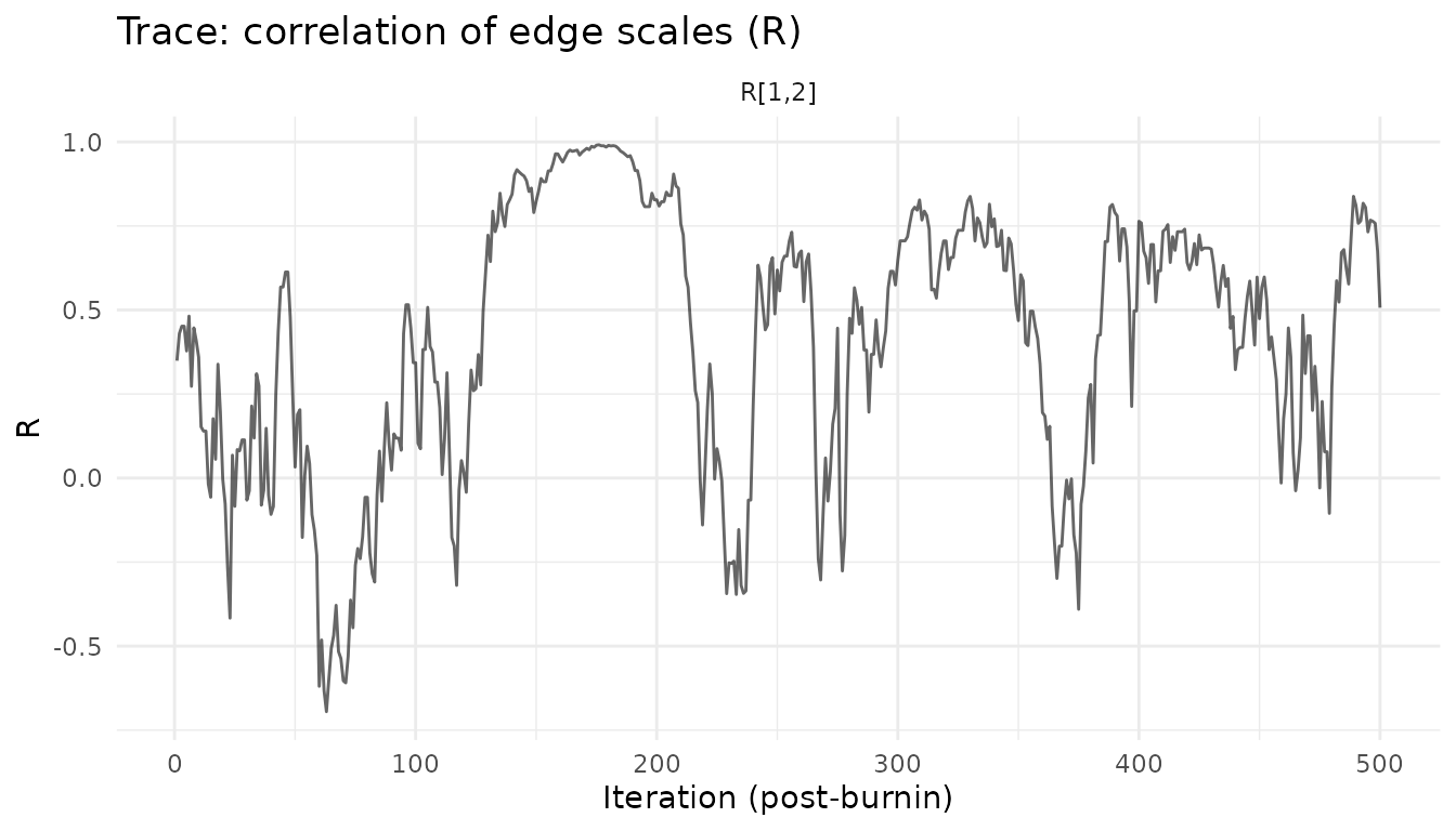

Differential edges and Bayesian FDR

diff_summary() gives one row per edge: the posterior mean and standard deviation of $D$ , a credible interval, and $P(|D| > c)$ for each threshold $c$ .

ds <- diff_summary(fit, scale = "pcor", deltas = c(0.05, 0.1))
head(ds[order(-ds$p_exceed_0.1), ])
#>     i  j       mean        sd         lower     median       upper
#> 6   3  4 -0.3527970 0.1249140 -0.5795079298 -0.3584738 -0.06939857
#> 65 10 12  0.3149062 0.1486431  0.0007256321  0.3302036  0.56660615
#> 1   1  2 -0.1994676 0.1791820 -0.5020627843 -0.1989438  0.17036425
#> 25  4  8  0.1830435 0.1415300 -0.0453670684  0.1937620  0.45110836
#> 66 11 12 -0.1210339 0.1649079 -0.4478402745 -0.1119946  0.21586969
#> 20  5  7 -0.1113987 0.1591270 -0.3962534596 -0.1102332  0.20513381
#>    excludes_zero p_sign p_exceed_0.05 p_exceed_0.1
#> 6           TRUE  0.994         0.984        0.968
#> 65          TRUE  0.976         0.926        0.892
#> 1          FALSE  0.860         0.878        0.774
#> 25         FALSE  0.894         0.808        0.718
#> 66         FALSE  0.780         0.758        0.616
#> 20         FALSE  0.748         0.750        0.606

select_diff_edges() selects the largest set of edges whose posterior expected false discovery rate is at most alpha:

sel <- select_diff_edges(fit, alpha = 0.05, delta = 0.1)
sel
#> <multiggm_diff_selection>
#>   Groups 1 vs 2, rule: magnitude (P(|D| > 0.1), pcor scale)
#>   Selected 1 edges at target FDR 0.05 (posterior expected FDR 0.032)
#>   i j  prob      mean
#> 1 3 4 0.968 -0.352797

Calibration caveat: do not use “the interval excludes zero”

It is tempting to call an edge differential when its credible interval for $D$ excludes zero, i.e. to run Bayesian FDR on $\max\{P(D > 0), P(D < 0)\}$ (the p_sign column). Under a continuous prior this is badly anti-conservative. $P(D = 0) = 0$ , so p_sign is not the probability that the edge differs. An edge with the same true value in both groups still has an estimated $D$ of sampling-noise size, and with large $n$ its posterior is concentrated enough to give p_sign near 1. In a simulation with p = 100 and n = 1000 per group, Bayesian FDR on p_sign gave an achieved FDR of about 0.50 at a nominal 0.05; the false calls were edges with identical true values whose $|D|$ was about 0.04 to 0.08.

The same applies to the SSVS sampler (its spike is a normal distribution) and to G-Wishart edges present in both groups.

Use $P(|D| > \delta)$ with a $\delta$ that is meaningful for your problem. The FDR is then controlled for the hypothesis $|D_{ij}| > \delta$ : a true difference smaller than $\delta$ counts as a null. For the indicator-based samplers, rule = "structural" ( $P(g_{1,ij} \ne g_{2,ij})$ ) is also available.

Memory, thinning and summary-only fits

Saved draws take $8 p^2 K \cdot$ nsave bytes per chain: 160 MB at p = 100, K = 2 and 1000 draws. Two ways to reduce this:

thin: the sampler runs every iteration but saves every thin-th draw.
save_draws = FALSE: no draws are kept. The sampler keeps running sums over every post-burn-in iteration of the posterior means and of $D$ (mean, SD, $P(D > 0)$ , $P(D < 0)$ and $P(|D| > c)$ for the thresholds in diff_deltas). coef(), fitted(), diff_summary() and select_diff_edges() use these; credible intervals and other draw-based functions are unavailable.

lean <- multiggm_mcmc(data_list = sim$data_list, method = "mghs",
                      burnin = 500, nsave = 500, nchains = 2, seed = 2,
                      save_draws = FALSE, diff_deltas = c(0.05, 0.1))
select_diff_edges(lean, alpha = 0.05, delta = 0.1)
#> <multiggm_diff_selection>
#>   Groups 1 vs 2, rule: magnitude (P(|D| > 0.1), pcor scale)
#>   Selected 1 edges at target FDR 0.05 (posterior expected FDR 0.019)
#>   i j  prob       mean
#> 1 3 4 0.981 -0.3619992

Chains are pooled by default in diff_summary() and select_diff_edges().

Stuck chains and run time

The sampler inherits a guard from the authors’ code: if a local-scale update would use parameters above $10^6$ , the chain is declared stuck. This happens when the global scale $\tau_k$ collapses or $R$ approaches a singular matrix, and it is more frequent for small, sparse problems. With p = 12 and n = 150 per group, 5 of 6 chains got stuck within 2,000 iterations, in both the authors’ code and this package. With n = 50, none of 6 did, and in a simulation study at p = 100 and n = 1000 all 100 fits completed, some after a restart. The package also checks every scale draw for non-finite values and caps every rejection loop, so a chain can no longer hang. A stuck chain is restarted from scratch (up to max_attempts, default 3) and the number of attempts is reported in summary(). If all attempts fail, multiggm_mcmc() stops with an error.

Run time per iteration depends strongly on the data, not only on $p$ : in our runs it ranged from about 10 to over 100 ms per iteration for $p \le 50$ .

References

Busatto, C. & Stingo, F.C. (2025). Inference of multiple high-dimensional networks with the Graphical Horseshoe prior. Journal of Computational and Graphical Statistics. doi:10.1080/10618600.2024.2435480

Busatto, C. & Stingo, F.C. (2025). The multiple graphical horseshoe: an application to breast cancer data. In SIS 2025, 435-440. Springer.

Li, Y., Craig, B.A. & Bhadra, A. (2019). The graphical horseshoe estimator for inverse covariance matrices. Journal of Computational and Graphical Statistics, 28(3), 747-757.

Newton, M.A., Noueiry, A., Sarkar, D. & Ahlquist, P. (2004). Detecting differential gene expression with a semiparametric hierarchical mixture method. Biostatistics, 5(2), 155-176.